Parameterized Kinetic Functionals

This example illustrates how we can extend the kinetic functional template class, KineticFunctional, to create parameterized functionals (e.g. neural network functionals), which can be fitted to data.

\(\mu\) TF + \(\lambda\) vW Functional and Linear Response Fitting

Let us start with a simple example to show how the KineticFunctional class can be used to define the \(\mu\) TF + \(\lambda\) vW functional.

class TFvW(KineticFunctional):

    def __init__(self, init_args=None):
        super().__init__()
        # init_args is a tuple
        if init_args is None:
            mu, lamb = 1, 1  # defauts to TF + vW
        else:
            mu, lamb = init_args
        # make µ and λ trainable parameters
        self.mu = torch.nn.Parameter(torch.tensor([mu], dtype=torch.double, device=self.device))
        self.lamb = torch.nn.Parameter(torch.tensor([lamb], dtype=torch.double, device=self.device))
        self.initialize()

    def forward(self, box_vecs, den):
        return self.mu * Weizsaecker(box_vecs, den) + self.lamb * ThomasFermi(box_vecs, den)

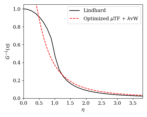
Now let us use the get_inv_G() utility function to fit the (\(\mu\), \(\lambda\)) parameters to reproduce the Lindhard function. (A simpler example of how the get_inv_G() function can be used can be found here.)

shape = (61, 61, 61)
box_vecs = 8 * torch.eye(3, dtype=torch.double)
den = torch.ones(shape, dtype=torch.double)

# compute Lindhard response function
eta, G_inv_lind = G_inv_lindhard(box_vecs, den)

# initialize µ TF + λ vW functional
TFvW_train = TFvW()
# set its parameters to have requires_grad = True to make them trainable
TFvW_train.param_grad(True)

print('Initial (µ, λ) = ({:.5g}, {:.5g})\n'.format(TFvW_train.mu.item(), TFvW_train.lamb.item()))

for i in range(20):
    eta, G_inv = get_inv_G(box_vecs, den, TFvW_train.forward, requires_grad=True)
    # computes the loss function and performs optimization to minimize it
    loss = TFvW_train.grid_error(G_inv_lind, G_inv)  # these are inherited helper functions from the
    TFvW_train.update_params(loss)                           # KineticFunctional class to facilitate training
    print('Epoch = {}, Loss = {:.5g}'.format(i, loss.item()))

TFvW_train.param_grad(False)

print('\nOptimized (µ, λ) = ({:.5g}, {:.5g})'.format(TFvW_train.mu.item(), TFvW_train.lamb.item()))

eta, G_inv_opt = get_inv_G(box_vecs, den, TFvW_train.forward)

# make plot to compare against Lindhard response
plt.rc('font', family='serif')
plt.subplots(figsize=(5, 4))

plt.plot(eta[0, 0, :], G_inv_lind[0, 0, :], '-k')
plt.plot(eta[0, 0, :], G_inv_opt[0, 0, :], '--r')

plt.xlim([0, eta[0, 0, -1]])
plt.ylim([0, 1.05])

plt.xlabel(r'$\eta$', fontsize=12)
plt.ylabel(r'$G^{-1}(\eta)$', fontsize=12)
plt.xticks(fontsize=12)
plt.yticks(fontsize=12)

labels = ['Lindhard', r'Optimized $\mu$TF + $\lambda$vW']
plt.legend(labels=labels, loc="upper right", borderaxespad=0.4, ncol=1, prop={'size': 12})

plt.tight_layout()
plt.show()

This results in

Initial (µ, λ) = (1, 1)

Epoch = 0, Loss = 0.0014799
Epoch = 1, Loss = 0.0011208
Epoch = 2, Loss = 0.00074545
Epoch = 3, Loss = 0.00059983
Epoch = 4, Loss = 0.00059983
Epoch = 5, Loss = 0.00060346
Epoch = 6, Loss = 0.00060346
Epoch = 7, Loss = 0.00057833
Epoch = 8, Loss = 0.00056777
Epoch = 9, Loss = 0.00056521
Epoch = 10, Loss = 0.00056278
Epoch = 11, Loss = 0.0005615
Epoch = 12, Loss = 0.00056022
Epoch = 13, Loss = 0.00056301
Epoch = 14, Loss = 0.00056301
Epoch = 15, Loss = 0.0005608
Epoch = 16, Loss = 0.0005603
Epoch = 17, Loss = 0.0005603
Epoch = 18, Loss = 0.00056026
Epoch = 19, Loss = 0.00056026

Optimized (µ, λ) = (0.70015, 0.60223)

and makes the plot

Neural Network Functional and Kinetic Potential Fitting

Let us now consider how the KineticFunctional class can be used to define a toy neural network functional. We use a simple Laplacian-level semi-local functional of the form

\[T_\text{S}[n] = T_\text{vW}[n] + \int_\Omega d^3\mathbf{r}~F_\text{enh}(s,q) \tau_\text{TF}(\mathbf{r})\]

where \(T_\text{vW}\) is the von Weizsaecker functional, \(\tau_\text{TF}(\mathbf{r})\) is the Thomas-Fermi kinetic energy density, \(s\) is the reduced gradient and \(q\) is the reduced Laplacian. We shall use a neural network to approximate the Pauli enhancement factor, \(F_\text{enh}(s,q)\).

class NeuralNetworkFunctional(KineticFunctional):

    def __init__(self, inner_layer_sizes):

        super().__init__()
        self.init_args = inner_layer_sizes
        layer_sizes = [2] + self.init_args + [1]

        self.nn = torch.nn.Sequential()
        for i in range(len(layer_sizes) - 1):
            self.nn.add_module('Linear_{}'.format(i), torch.nn.Linear(layer_sizes[i], layer_sizes[i + 1],
                               dtype=torch.double))
            if i != len(layer_sizes) - 2:
                self.nn.add_module('Activation_{}'.format(i), torch.nn.SiLU())
        self.nn.add_module('Activation_-1', torch.nn.Softplus())
        self.initialize()

    def forward(self, box_vecs, den):
        # getting descriptors
        kx, ky, kz, k2 = wavevecs(box_vecs, den.shape)
        s = reduced_gradient(kx, ky, kz, den)
        q = reduced_laplacian(k2, den)

        # compute Pauli enhancement factor
        Fenh = torch.squeeze(self.nn(torch.cat((s.unsqueeze(-1), q.unsqueeze(-1)), dim=-1)))

        # assembling the terms
        vol = torch.abs(torch.linalg.det(box_vecs))
        TF_ked = 0.3 * (3 * np.pi * np.pi)**(2 / 3) * den.pow(5 / 3)
        Pauli_T = torch.mean(Fenh * TF_ked) * vol
        return Weizsaecker(box_vecs, den) + Pauli_T

We now give an example of how the get_functional_derivative() utility function can be used to facilitate the fitting of this neural network functional’s functional derivative (or kinetic potential) to some reference kinetic potential. (A simpler example of how the get_functional_derivative() function can be used can be found here.) As this is just a toy model to illustrate how one might use PROFESS-AD’s utilities for such training, we shall fit the neural network functional’s kinetic potential to that of the Wang-Teter functional’s for a face-centred cubic (fcc) aluminium system, where the density was optimized using the Wang-Teter functional. Of course, this is just a toy example to explain how PROFESS-AD can be used for such training - it is uncertain if the model trained is transferable enough to be used for density optimizations due to overfitting on a single example.

# generate an optimized density to be used
terms = [IonIon, IonElectron, Hartree, WangTeter, PerdewBurkeErnzerhof]
box_vecs, frac_ion_coords = get_cell('fcc', vol_per_atom=16.9, coord_type='fractional')
ions = [['Al', 'al.gga.recpot', frac_ion_coords]]
shape = System.ecut2shape(2000, box_vecs)
system = System(box_vecs, shape, ions, terms, units='a', coord_type='fractional')
system.optimize_density(ntol=1e-10)

# extract optimized density and lattice vectors (in atomic units)
den = system.density()
box_vecs = system.lattice_vectors('b')

# as a toy example, let's try to fit the neural network functional's kinetic potential
# to that of the Wang-Teter functional for this optimized density

# the "target"
WT_kp = get_functional_derivative(box_vecs, den, WangTeter)

# create the neural network functional with 3 hidden layers having 8 nodes each
model = NeuralNetworkFunctional([8, 8, 8])

# explicitly defining the optimizer and its parameters
model.optimizer = torch.optim.Rprop(model.parameters(), lr=0.01, step_sizes=(1e-8, 50))

model.param_grad(True)

for iter in range(201):
    NN_kp = get_functional_derivative(box_vecs, den, model.forward, requires_grad=True)
    loss = model.grid_error(WT_kp, NN_kp)
    model.update_params(loss)
    if iter % 20 == 0:
        print('Iteration {}, RMSE = {:.5g}'.format(iter, torch.sqrt(loss).item()))

model.param_grad(False)

NN_kp = get_functional_derivative(box_vecs, den, model.forward)

# make plot
plt.rc('font', family='serif')
fig, axs = plt.subplots(figsize=(5, 5), nrows=2, sharex=True, gridspec_kw={'hspace': 0})

r = np.linspace(0, 1, shape[0])
axs[0].plot(r, [den[i, i, i] for i in range(den.shape[0])], '-k')

axs[1].plot(r, [WT_kp[i, i, i] for i in range(den.shape[0])], '-b')
axs[1].plot(r, [NN_kp[i, i, i] for i in range(den.shape[0])], '--r')

axs[0].set_xlim([0, 1])
axs[1].set_xlim([0, 1])

axs[0].set_ylabel('Electron Density (a.u.)')
axs[1].set_ylabel('Kinetic Potential (a.u.)')
axs[1].set_xlabel(r'[111] direction ($a_0 \sqrt{3}$)')

labels = ['WT', 'NN']
plt.legend(labels=labels, loc="lower center", borderaxespad=0.4, ncol=1, prop={'size': 10})

plt.tight_layout()
plt.show()

This results in

Iteration 0, RMSE = 0.1618
Iteration 20, RMSE = 0.05397
Iteration 40, RMSE = 0.029365
Iteration 60, RMSE = 0.022676
Iteration 80, RMSE = 0.021627
Iteration 100, RMSE = 0.020801
Iteration 120, RMSE = 0.020157
Iteration 140, RMSE = 0.019637
Iteration 160, RMSE = 0.01925
Iteration 180, RMSE = 0.018822
Iteration 200, RMSE = 0.018475

and makes the plot

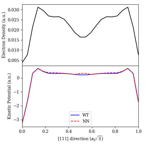
As the neural network parameters are initialized randomly, running the above code may lead to different results each time.